Note
Go to the end to download the full example code.
Cardio-respiratory synchronization
RespHRV is not the only form of cardio-respiratory coupling. Bartsch et al, 2012 (https://doi.org/10.1073/pnas.1204568109) described another form that they called the cardio-respi phase synchronisation (CRPS). CRPS leads to clustering of heartbeats at certain phases of the breathing cycle. We developed a way of studying such coupling that is presented in this example
import numpy as np
import matplotlib.pyplot as plt
from pathlib import Path
from pprint import pprint

import physio
Read data
For this tutorial, we will use an internal file stored in NumPy format for demonstration purposes.
See Getting started tutorial, first section, for a description of
the capabilities of physio for reading raw data formats.
raw_resp = np.load('resp2_airflow.npy') # load respi
raw_ecg = np.load('ecg2.npy') # load ecg
srate = 1000. # our example signals have been recorded at 1000 Hz

times = np.arange(raw_resp.size) / srate # build time vector
Get respiratory cycles and ECG peaks using parameter_preset, and compute instantaneous heart rate
See Respiration tutorial and
ECG tutorial for a detailed explanation of how to use
compute_respiration() and compute_ecg(), respectively.
resp, resp_cycles = physio.compute_respiration(raw_resp, srate, parameter_preset='human_airflow') # set 'human_airflow' as preset because example resp is an airflow from human
ecg, ecg_peaks = physio.compute_ecg(raw_ecg, srate, parameter_preset='human_ecg') # set 'human_ecg' as preset because example ecg is from human
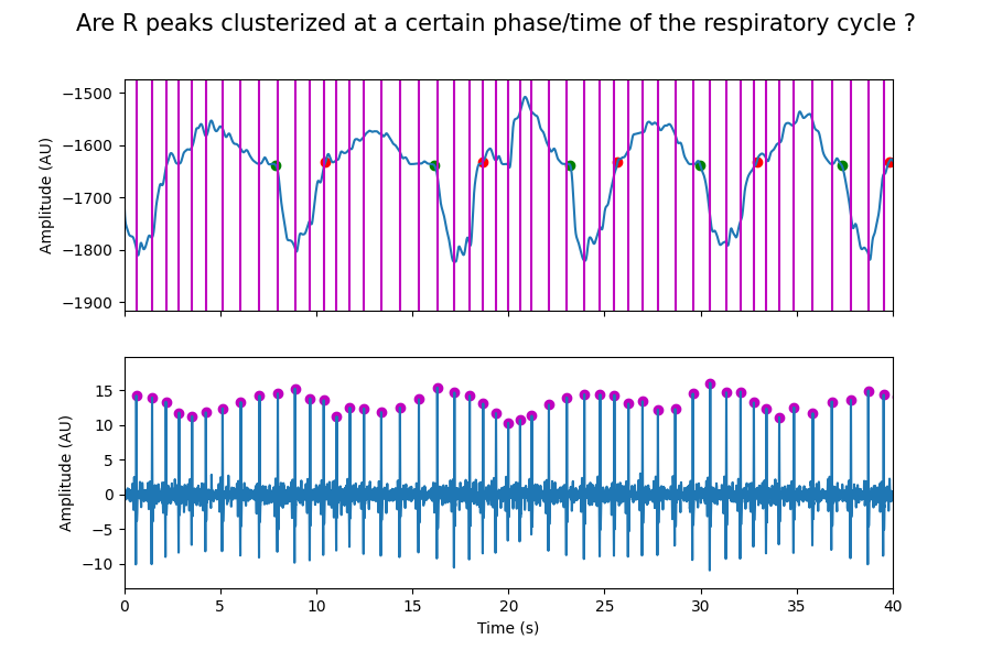
A first plot to explore the question
fig, axs = plt.subplots(nrows=2, sharex=True, figsize=(9, 6))
fig.suptitle('Are R peaks clusterized at a certain phase/time of the respiratory cycle ?', fontsize = 15)

ax = axs[0]
ax.plot(times, resp)
ax.scatter(resp_cycles['inspi_time'], resp[resp_cycles['inspi_index']], color='g')
ax.scatter(resp_cycles['expi_time'], resp[resp_cycles['expi_index']], color='r')
for t in ecg_peaks['peak_time']:
    ax.axvline(t, color='m')
ax.set_ylabel('Amplitude (AU)')

ax = axs[1]
ax.plot(times, ecg)
ax.scatter(ecg_peaks['peak_time'], ecg[ecg_peaks['peak_index']], color='m')
ax.set_xlabel('Time (s)')
ax.set_ylabel('Amplitude (AU)')

ax.set_xlim(0,  40)
(0.0, 40.0)
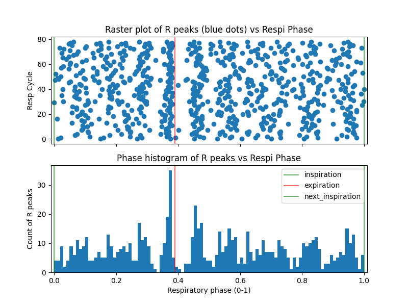
Phase synchronization : from ECG peak times to respiratory phase
time_to_cycle() is the key function that transforms
the times of ECG R peaks into phases of respiratory cycles.
To use this function, you must provide:
times: np.array. Timings in seconds of ECG R peaks (ecg_peaks[‘peak_time’].values).
cycle_times: np.ndarray. Respiratory cycle times (resp_cycles[[‘inspi_time’, ‘expi_time’, ‘next_inspi_time’]].values). See Respiration tutorial for details on detected respiratory cycle features.
segment_ratios: None, float, or list of floats.
None → 1 segment.
Float or list of floats → 2 segments.
List of floats → more than 2 segments.
This defines the ratio (between 0 and 1) at which the cycle is divided. In practice, this is the phase ratio of the inhalation-to-exhalation transition. It can be computed, for example, with resp_cycles[‘cycle_ratio’].median().
The function returns rpeak_phase, the R peak times converted to respiratory phases as floats:
Example: 4.32 means that the current R peak occurred during the 4th respiratory cycle at 32% of its duration.
Pooled phases can be obtained using modulo 1 and represented on a raster plot or as a phase histogram.
inspi_ratio = resp_cycles['cycle_ratio'].median()

cycle_times = resp_cycles[['inspi_time', 'expi_time', 'next_inspi_time']].values

rpeak_phase = physio.time_to_cycle(ecg_peaks['peak_time'].values, cycle_times, segment_ratios=[inspi_ratio])


count, bins = np.histogram(rpeak_phase % 1, bins=np.linspace(0, 1, 101)) # modulo 1

fig, axs = plt.subplots(nrows=2, sharex=True, figsize=(8, 6))
ax = axs[0]
ax.scatter(rpeak_phase % 1, np.floor(rpeak_phase))
ax.set_ylabel('Resp Cycle')
ax.set_title('Raster plot of R peaks (blue dots) vs Respi Phase')

ax = axs[1]
ax.bar(bins[:-1], count, width=bins[1] - bins[0], align='edge')
ax.set_xlabel('Respiratory phase (0-1)')
ax.set_ylabel('Count of R peaks')
ax.set_title('Phase histogram of R peaks vs Respi Phase')

for ax in axs:
    ax.axvline(0, color='g', label='inspiration', alpha=.6)
    ax.axvline(inspi_ratio, color='r', label='expiration', alpha=.6)
    ax.axvline(1, color='g', label='next_inspiration', alpha=.6)
ax.legend()
ax.set_xlim(-0.01, 1.01)
(-0.01, 1.01)
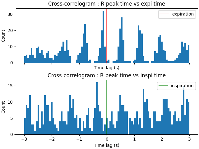
Time synchronization : Cross-correlogram between expiration/inspiration times and ECG peak times
Another way to explore the preferential clustering of R peaks is to compare their timing to specific respiratory cycle times, such as inspiration or expiration.
The key function is crosscorrelogram().
To use this function, you must provide:
a: R peak times (ecg_peaks[‘peak_time’].values).
b: Respiratory times. Use resp_cycles[‘expi_time’].values to compare R peak times to expiration times, or resp_cycles[‘inspi_time’].values to compare them to inspiration times.
bins: np.array. The histogram bins, which must be centered around 0 and span a range of seconds approximately equal to cycle durations.
When called, this function:
Computes the combinatorial differences between all R peak times and all given respiratory times.
Binarizes the obtained time differences according to the provided bins.
A histogram can then be plotted to reveal possible non-uniformity in the distribution, indicating the “attraction” of R peaks to a given respiratory time. The less flat it is—and the more it is organized as oscillations—the more likely there is cardio-respiratory synchronization.
bins = np.linspace(-3, 3, 100)


count, bins = physio.crosscorrelogram(ecg_peaks['peak_time'].values,
                               resp_cycles['expi_time'].values,
                               bins=bins)

fig, axs = plt.subplots(nrows=2, sharex=True, constrained_layout = True)
ax = axs[0]
ax.bar(bins[:-1], count, align='edge', width=bins[1] - bins[0])
ax.set_xlabel('Time lag (s)')
ax.set_ylabel('Count')
ax.axvline(0, color='r', label='expiration', alpha=.6)
ax.legend(loc = 'upper right')
ax.set_title('Cross-correlogram : R peak time vs expi time')


ax = axs[1]
count, bins = physio.crosscorrelogram(ecg_peaks['peak_time'].values,
                               resp_cycles['inspi_time'].values,
                               bins=bins)
ax.bar(bins[:-1], count, align='edge', width=bins[1] - bins[0])
ax.set_xlabel('Time lag (s)')
ax.set_ylabel('Count')
ax.axvline(0, color='g', label='inspiration', alpha=.6)
ax.legend(loc = 'upper right')
ax.set_title('Cross-correlogram : R peak time vs inspi time')


plt.show()
Total running time of the script: (0 minutes 0.892 seconds)