Note
Go to the end to download the full example code.
Respiration tutorial
import numpy as np
import matplotlib.pyplot as plt
from pathlib import Path
from pprint import pprint

import physio
Respiration cycle detection. The faster way: using parameter_preset.
The fastest way to process respiration with physio is to use compute_respiration() which is a high-level wrapper function that simplifies respiratory signal analysis.
To use this function, you must provide:
raw_resp : the raw respiratory signal as a NumPy array.
srate : the sampling rate of the respiratory signal
parameter_preset : a string specifying the type of respiratory data, which determines the set of parameters used for processing. Can be one of: human_airflow, human_co2, human_belt, rat_plethysmo, or rat_etisens_belt.
When called, compute_respiration() performs the following:
Preprocesses the respiratory signal (returns a NumPy array: resp)
Computes cycle-by-cycle features (returns a pd.DataFrame: resp_cycles)
Warning: The orientation of the raw_resp trace is important (multiply it by -1 for reversing it if necessary).
Inspiration must point downward for human_airflow or human_co2,
because downward deflections are interpreted by compute_respiration() as inspiration.
For rat_plethysmo or rat_etisens_belt, the inspiration–expiration transition must point upward.
For this tutorial, we will use an internal file already stored in NumPy format for demonstration purposes.
raw_resp = np.load('resp1_airflow.npy') # load respi
srate = 1000. # our example signals have been recorded at 1000 Hz

times = np.arange(raw_resp.size) / srate # build time vector


# the easiest way is to use predefined parameters
resp, resp_cycles = physio.compute_respiration(raw_resp, srate, parameter_preset='human_airflow')  # set 'human_airflow' as preset because example resp is an airflow from humans

# resp_cycles is a dataframe containing all cycles and related features (duration, amplitude, volume, timing, etc...).
print(resp_cycles)

inspi_ind = resp_cycles['inspi_index'].values # get index of inspiration start points
expi_ind = resp_cycles['expi_index'].values # get index of expiration start points

fig, ax = plt.subplots()
ax.plot(times, raw_resp)
ax.plot(times, resp)
ax.scatter(times[inspi_ind], resp[inspi_ind], color='green', label = 'inspiration start')
ax.scatter(times[expi_ind], resp[expi_ind], color='red', label = 'expiration start')
ax.set_xlabel('Time (s)')
ax.set_ylabel('Amplitude (AU)')
ax.set_ylim(-1750, -1450)
ax.set_title('Respiratory cycle detection')
ax.legend(loc = 'upper right')

ax.set_xlim(110, 170)

    inspi_index  expi_index  ...  expi_peak_time  total_volume
0           963        3849  ...           4.969    291.424431
1          8755       12470  ...          13.479    248.679461
2         16629       20085  ...          20.995    225.343872
3         25589       28826  ...          30.576    180.226656
4         35467       39250  ...          41.144    218.772816
5         45631       48992  ...          50.698    185.303221
6         55914       59772  ...          61.809    222.938344
7         67325       70801  ...          72.750    173.728543
8         78023       81420  ...          82.834    241.129370
9         86030       89213  ...          90.996    162.205566
10        94623       97972  ...         100.891   1083.803965
11       104423      108683  ...         110.518    237.217117
12       114252      117877  ...         119.319    216.113417
13       124700      127879  ...         129.999    227.066006
14       134461      138178  ...         140.396    196.708830
15       145780      149124  ...         151.674    145.025697
16       156359      159809  ...         161.764    173.603192
17       165930      169247  ...         171.542    179.954129
18       175415      178225  ...         180.364    129.920402
19       184867      188712  ...         190.757    172.982517
20       195179      199483  ...         201.509    187.120995
21       205152      209074  ...         210.793    218.716716
22       214162      217778  ...         220.553    206.830544
23       223497      227737  ...         229.680    222.818645
24       233353      237747  ...         239.786    254.319332
25       242949      247667  ...         249.696    318.826908
26       253240      257182  ...         259.468    258.070059
27       263116      266749  ...         269.279    204.821141
28       273102      277759  ...         279.953    244.363774
29       284946      288731  ...         291.162    189.545873

[30 rows x 21 columns]

(110.0, 170.0)
What is parameter_preset ?
Using parameter_preset tells compute_respiration() to process respiration
according to a predefined set of parameters already optimized by physio.
To get an idea of the default parameters used in parameter_preset,
you can call get_respiration_parameters().
Here is an example showing the set of parameters applied in the case of a human airflow signal.
parameters = physio.get_respiration_parameters('human_airflow') # parameters is a nested dictionary of parameters used at each processing step.
pprint(parameters) # pprint to "pretty print"
{'baseline': {'baseline_mode': 'median'},
 'cycle_clean': {'low_limit_log_ratio': 4.5,
                 'variable_names': ['inspi_volume', 'expi_volume']},
 'cycle_detection': {'epsilon_factor1': 10.0,
                     'epsilon_factor2': 5.0,
                     'inspiration_adjust_on_derivative': False,
                     'method': 'crossing_baseline'},
 'preprocess': {'band': 7.0, 'btype': 'lowpass', 'ftype': 'bessel', 'order': 5},
 'sensor_type': 'airflow',
 'smooth': {'sigma_ms': 60.0, 'win_shape': 'gaussian'}}
Tuning parameters if unsatisfied
Variability during data acquisition (subject, acquisition system) can affect the recorded respiratory signal.
Such variability may make some predefined parameters of physio inappropriate.
In this situation, you can tune certain parameters by re-assigning values to the keys of the parameters dictionary. You may also tune multiple parameters at once if necessary.
To fine-tune parameters properly, a good understanding of each parameter’s role is required. For this reason, we have dedicated a whole section to this topic — see the “Parameters” section.
For example, here we modify the length of the smoothing parameter, which corresponds to the duration in milliseconds of the Gaussian smoothing kernel (the width of the bell-shaped curve), usually referred to as sigma.
# let's change one parameter in the nested structure ...
parameters['smooth']['sigma_ms'] = 100. # at the key "smooth" and the sub-key "sigma_ms", the default values is 60. Here we replace it by 100 milliseconds to induce more smoothing
pprint(parameters) # pprint to "pretty print"

# ... and use them by providing it to "parameters"
resp, resp_cycles = physio.compute_respiration(raw_resp, srate, parameters=parameters) # preset_parameters = None in this case, because parameters is now explicitly defined
{'baseline': {'baseline_mode': 'median'},
 'cycle_clean': {'low_limit_log_ratio': 4.5,
                 'variable_names': ['inspi_volume', 'expi_volume']},
 'cycle_detection': {'epsilon_factor1': 10.0,
                     'epsilon_factor2': 5.0,
                     'inspiration_adjust_on_derivative': False,
                     'method': 'crossing_baseline'},
 'preprocess': {'band': 7.0, 'btype': 'lowpass', 'ftype': 'bessel', 'order': 5},
 'sensor_type': 'airflow',
 'smooth': {'sigma_ms': 100.0, 'win_shape': 'gaussian'}}
Using low-level functions to control each step of the pipeline
compute_respiration() is a high-level wrapper function that simplifies respiratory signal analysis.
However, you may want more control over the entire process and therefore use the low-level functions of physio.
Here are the details of all low-level functions used internally by compute_respiration().
resp = physio.preprocess(raw_resp, srate, band=25., btype='lowpass', ftype='bessel', order=5, normalize=False) # filter
resp = physio.smooth_signal(resp, srate, win_shape='gaussian', sigma_ms=90.0) # smooth

baseline = physio.get_respiration_baseline(resp, srate, baseline_mode='median') # compute baseline level
print('baseline :', baseline)

# this will give a numpy.array with shape (num_cycle, 3)
cycles = physio.detect_respiration_cycles(resp, srate, baseline_mode='manual', baseline=baseline) # detect inspi-expi / expi-inspi / next inspi-expi indices
print(cycles[:10])

# this will return a dataframe with all cycles and features before cleaning
resp_cycles = physio.compute_respiration_cycle_features(resp, srate, cycles, baseline=baseline, sensor_type = 'airflow') # compute cycle-by-cycle resp features on airflow sensor type

# this will remove outliers cycles based on log ratio distribution
resp_cycles = physio.clean_respiration_cycles(resp, srate, resp_cycles, baseline, low_limit_log_ratio=4.5, sensor_type = 'airflow') # clean features
print(resp_cycles.head(10))


inspi_ind = resp_cycles['inspi_index'].values # get index of inspiration start points
expi_ind = resp_cycles['expi_index'].values # get index of expiration start points

fig, ax = plt.subplots()
ax.plot(times, resp, label = 'preprocessed resp signal')
ax.scatter(times[inspi_ind], resp[inspi_ind], marker='o', color='green', label = 'inspiration start')
ax.scatter(times[expi_ind], resp[expi_ind], marker='o', color='red', label = 'expiration start')
ax.axhline(baseline, color='Coral', label = 'baseline', ls = '--', alpha = 0.9)
ax.set_ylabel('Amplitude (AU)')
ax.set_xlabel('Time (s)')
ax.set_title('Respiratory cycle detection (using low-level functions)')
ax.set_ylim(-1750, -1450)
ax.set_xlim(110, 170)
ax.legend(loc = 'upper right')

plt.show()

baseline : -1635.636336457686
[[  959  3856  8749]
 [ 8749 12461 16623]
 [16623 20084 25584]
 [25584 28837 35465]
 [35465 39256 45628]
 [45628 48997 55907]
 [55907 59779 67319]
 [67319 70804 78017]
 [78017 81433 86026]
 [86026 89212 94617]]
/home/docs/checkouts/readthedocs.org/user_builds/physio/envs/stable/lib/python3.11/site-packages/physio/respiration.py:701: UserWarning: clean_respiration_cycles() need variable_names to be set, variable_name=['inspi_volume', 'expi_volume'] is set to  for backward compatibility
  warnings.warn("clean_respiration_cycles() need variable_names to be set, variable_name=['inspi_volume', 'expi_volume'] is set to  for backward compatibility")
   inspi_index  expi_index  ...  expi_peak_time  total_volume
0          959        3856  ...           4.968    291.387502
1         8749       12461  ...          13.477    248.663272
2        16623       20084  ...          20.993    225.308920
3        25584       28837  ...          30.575    180.185173
4        35465       39256  ...          41.138    218.718159
5        45628       48997  ...          50.699    185.262616
6        55907       59779  ...          61.812    222.891807
7        67319       70804  ...          72.757    173.670636
8        78017       81433  ...          82.837    241.081997
9        86026       89212  ...          90.998    162.158526

[10 rows x 21 columns]
Respiration features / metrics
resp_cycles is a dataframe containing one row per respiratory cycle and one column per feature. Depending on the sensor type, each cycle is described by multiple features.
Some features are related to the position (index) or time of particular points within the cycle:
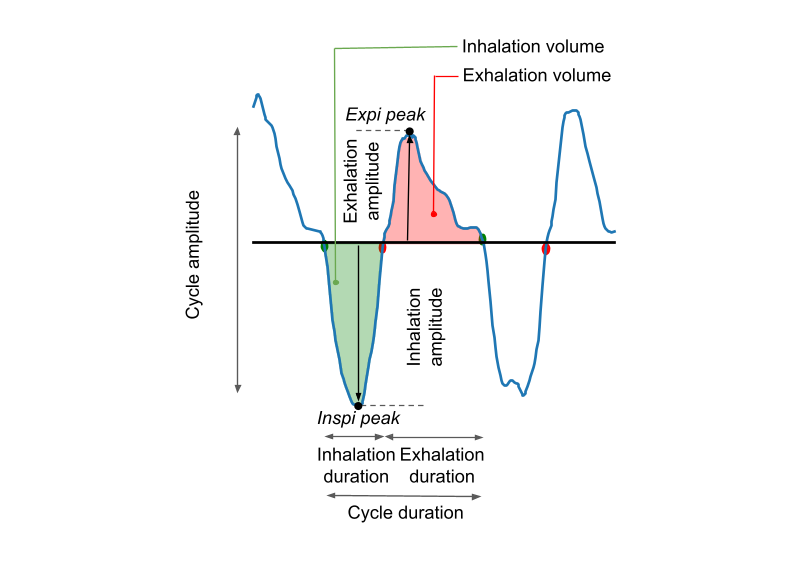
inspi_index: Index of the start of inspiration (green point in the figure below). The index refers to the sequential position of the sample in the entire respiratory time series.
expi_index: Index of the start of expiration (red point in the figure below).
next_inspi_index: Index of the start of the next inspiration (equal to the inspi_index of cycle n+1).
inspi_time: (units = s) Time of the start of inspiration (green point in the figure below).
expi_time: (units = s) Time of the start of expiration (red point in the figure below).
next_inspi_time: (units = s) Time of the start of the next inspiration.
inspi_peak_index: Index of the inspiratory peak = position of the minimum sample of the cycle in the respiratory time series (computed only if sensor_type = airflow).
expi_peak_index: Index of the expiratory peak = position of the maximum sample of the cycle in the respiratory time series (computed only if sensor_type = airflow).
inspi_peak_time: (units = s) Time of the inspiratory peak = timestamp of the minimum sample of the cycle (computed only if sensor_type = airflow).
expi_peak_time: (units = s) Time of the expiratory peak = timestamp of the maximum sample of the cycle (computed only if sensor_type = airflow).
From these points, many derived features of interest (e.g., for statistics) are computed:
cycle_duration: (units = s) Duration of the cycle in seconds = next_inspi_time - inspi_time
inspi_duration: (units = s) Duration of inspiration in seconds = expi_time - inspi_time
expi_duration: (units = s) Duration of expiration in seconds = next_inspi_time - expi_time
cycle_freq: (units = Hz) Breathing frequency in Hertz = 1 / cycle_duration
cycle_ratio: (units = AU because proportion) Ratio of inspiration duration to total cycle duration = inspi_duration / cycle_duration. Equivalent to the relative position of the transition from inspiration to expiration.
inspi_amplitude: (units = AU, the units of the recorded respiratory signal) Amplitude difference of the respiratory signal from baseline at inspi_peak_index (computed only if sensor_type = airflow or belt). Equivalent to peak inspiratory flow (black descending arrow in the figure below).
expi_amplitude: (units = AU, the units of the recorded respiratory signal) Amplitude difference of the respiratory signal from baseline at expi_peak_index (computed only if sensor_type = airflow’ or belt). Equivalent to peak expiratory flow (black ascending arrow in the figure below).
total_amplitude: (units = AU, the units of the recorded respiratory signal) Sum of inspi_amplitude + expi_amplitude (computed only if sensor_type = airflow or belt).
inspi_volume: (units = AU * s, depending on units the recorded respiratory signal) Integral of the respiratory signal below baseline during inspiration (computed only if sensor_type = airflow). Equivalent to the green area in the figure below.
expi_volume: (units = AU * s, depending on units the recorded respiratory signal) Integral of the respiratory signal above baseline during expiration (computed only if sensor_type = airflow). Equivalent to the red area in the figure below.
total_volume: (units = AU * s, depending on units the recorded respiratory signal) Sum of inspi_volume + expi_volume (computed only if sensor_type = airflow). Equivalent to the sum of the green + red areas in the figure below.
pprint(f'{resp_cycles.shape[0]} detected cycles')
pprint(f'{resp_cycles.shape[1]} computed features, which are the following :')
pprint(resp_cycles.columns.to_list())
'30 detected cycles'
'21 computed features, which are the following :'
['inspi_index',
 'expi_index',
 'next_inspi_index',
 'inspi_time',
 'expi_time',
 'next_inspi_time',
 'cycle_duration',
 'inspi_duration',
 'expi_duration',
 'cycle_freq',
 'cycle_ratio',
 'inspi_volume',
 'expi_volume',
 'total_amplitude',
 'inspi_amplitude',
 'expi_amplitude',
 'inspi_peak_index',
 'expi_peak_index',
 'inspi_peak_time',
 'expi_peak_time',
 'total_volume']
Quick example with respiration recorded using a belt
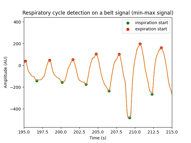
For this tutorial, we will use an internal file already stored in NumPy format for demonstration purposes. This file corresponds to 5 minutes of signal recorded with a belt on a human subject. The belt is a sensor of trunk circumference: the signal rises when the trunk dilates and decreases when the trunk retracts.
Therefore, the detection method does not rely on a “baseline-crossing” approach, but rather on a “min-max” approach. This min_max method is activated via the parameter_preset dedicated to this situation.
Note that respiratory signals recorded with belts are often of poor quality. In addition, some participants may present paradoxical respiration, with the trunk retracting during inspiration and dilating during expiration. In such cases, the metrics returned in resp_cycles_belt will not be meaningful.
Further note that in case of a belt, volumes can’t be computed and amplitudes are no the same ones than in airflow. In this case this a max - min measure related to a circumference, while in case of an airflow this is a vertical distance to the baseline… meaning an instantaneous flow.
Let’s run a short example.
raw_resp_belt = np.load('resp3_belt.npy') # load respi belt
srate = 1000. # our example signals have been recorded at 1000 Hz

times = np.arange(raw_resp_belt.size) / srate # build time vector


# the easiest way is to use predefined parameters
resp_belt, resp_cycles_belt = physio.compute_respiration(raw_resp_belt, srate, parameter_preset='human_belt')  # set 'human_belt' as preset because example resp is an airflow from humans

# print human_belt params
pprint(physio.get_respiration_parameters('human_belt'))

# resp_cycles_belt is a dataframe containing all cycles and related features (duration, amplitude, timing, etc...). In the case of belt, volumes are not computed.
print(resp_cycles_belt)

inspi_ind = resp_cycles_belt['inspi_index'].values # get index of inspiration start points
expi_ind = resp_cycles_belt['expi_index'].values # get index of expiration start points

fig, ax = plt.subplots()
ax.plot(times, raw_resp_belt)
ax.plot(times, resp_belt)
ax.scatter(times[inspi_ind], resp_belt[inspi_ind], color='green', label = 'inspiration start')
ax.scatter(times[expi_ind], resp_belt[expi_ind], color='red', label = 'expiration start')
ax.set_xlim(195, 215)
ax.set_xlabel('Time (s)')
ax.set_ylabel('Amplitude (AU)')
ax.set_title('Respiratory cycle detection on a belt signal (min-max signal)')
ax.legend(loc = 'upper right')
{'baseline': None,
 'cycle_clean': {'low_limit_log_ratio': 8.0,
                 'variable_names': ['inspi_amplitude', 'expi_amplitude']},
 'cycle_detection': {'exclude_sweep_ms': 200.0, 'method': 'min_max'},
 'preprocess': {'band': 5.0, 'btype': 'lowpass', 'ftype': 'bessel', 'order': 5},
 'sensor_type': 'belt',
 'smooth': {'sigma_ms': 40.0, 'win_shape': 'gaussian'}}
    inspi_index  expi_index  ...  inspi_amplitude  expi_amplitude
0          3875        6168  ...       497.761465      747.099189
1          9499       11176  ...       453.815590      316.429352
2         13317       15405  ...       390.832924      432.101417
3         18137       19825  ...       389.225680      436.079255
4         22469       24252  ...       479.711632      414.107313
..          ...         ...  ...              ...             ...
82       283479      284539  ...       256.353191      236.941509
83       286221      287424  ...       250.333176      273.552655
84       289046      290081  ...       287.955141      288.775000
85       291656      292918  ...       284.711136      271.157089
86       294552      295610  ...       271.450497      285.710228

[87 rows x 13 columns]

<matplotlib.legend.Legend object at 0x739061bd40d0>
Quick example with respiration recorded using a CO2 sensor
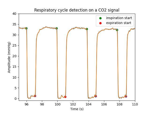
For this tutorial, we will use an internal file already stored in NumPy format for demonstration purposes. This file corresponds to 5 minutes of signal recorded with a CO2 sensor at 60 Hz from a human subject.
In the upper airways, CO2 concentration decreases during inspiration and increases during exhalation, and so does the recorded signal.
Therefore, the detection method does not rely on a “baseline-crossing” approach, but rather on a dedicated “co2” method. This method is activated via the parameter_preset specific to this situation.
Note that for co2, amplitude and volumes are not computed.
Let’s run a short example.
raw_resp_co2 = np.load('resp4_CO2.npy') # load respi co2
srate = 60. # our example signals have been recorded at 60 Hz

times = np.arange(raw_resp_co2.size) / srate # build time vector


# the easiest way is to use predefined parameters
resp_co2, resp_cycles_co2 = physio.compute_respiration(raw_resp_co2, srate, parameter_preset='human_co2')  # set 'human_co2' as preset because example resp is an airflow from humans

# print human_co2 params
pprint(physio.get_respiration_parameters('human_co2'))

# resp_cycles_co2 is a dataframe containing all cycles and related features (duration, timing, etc...). In the case of belt, volumes and amplitudes are not computed.
print(resp_cycles_co2)

inspi_ind = resp_cycles_co2['inspi_index'].values # get index of inspiration start points
expi_ind = resp_cycles_co2['expi_index'].values # get index of expiration start points

fig, ax = plt.subplots()
ax.plot(times, raw_resp_co2)
ax.plot(times, resp_co2)
ax.scatter(times[inspi_ind], resp_co2[inspi_ind], color='green', label = 'inspiration start')
ax.scatter(times[expi_ind], resp_co2[expi_ind], color='red', label = 'expiration start')
ax.set_xlim(95, 110)
ax.set_ylim(-1, 40)
ax.set_xlabel('Time (s)')
ax.set_ylabel('Amplitude (mmHg)')
ax.set_title('Respiratory cycle detection on a CO2 signal')
ax.legend(loc = 'upper right')
{'baseline': None,
 'cycle_clean': None,
 'cycle_detection': {'clean_by_mid_value': True,
                     'method': 'co2',
                     'thresh_expi_factor': 0.05,
                     'thresh_inspi_factor': 0.08},
 'preprocess': {'band': 10.0,
                'btype': 'lowpass',
                'ftype': 'bessel',
                'order': 5},
 'sensor_type': 'co2',
 'smooth': {'sigma_ms': 40.0, 'win_shape': 'gaussian'}}
    inspi_index  expi_index  ...  cycle_freq  cycle_ratio
0           131         198  ...    0.255319     0.285106
1           366         396  ...    0.256410     0.128205
2           600         667  ...    0.256410     0.286325
3           834         865  ...    0.255319     0.131915
4          1069        1136  ...    0.255319     0.285106
..          ...         ...  ...         ...          ...
76        17755       17821  ...    0.256410     0.282051
77        17989       18055  ...    0.300000     0.330000
78        18189       18258  ...    0.256410     0.294872
79        18423       18491  ...    0.254237     0.288136
80        18659       18688  ...    0.740741     0.358025

[81 rows x 11 columns]

<matplotlib.legend.Legend object at 0x739061a82990>
Total running time of the script: (0 minutes 0.677 seconds)