RespHRV Tutorial

Respiratory Heart Rate Variability (RespHRV; previously called Respiratory Sinus Arrhythmia, RSA — see this paper explaining the redefinition of the term: 10.1038/s41569-025-01160-z) can be analyzed using the physio toolbox, which provides an innovative method to extract features from heart rate dynamics on a respiratory cycle-by-cycle basis.

The method consists of:

• Detecting respiratory cycles

• Detecting ECG peaks

• Computing instantaneous heart rate in beats per minute

• Extracting features of this heart rate time series for each respiratory cycle

• Using cyclic deformation of the heart rate time series and stacking all epochs

This method has two important advantages:

• RespHRV features can be finely obtained for each respiratory cycle

• Heart rate dynamics can be analyzed at each phase bin of the respiratory cycle

import numpy as np
import matplotlib.pyplot as plt
import pandas as pd
from pathlib import Path
from pprint import pprint
from scipy import stats

import physio

Read data

For this tutorial, we will use an internal file stored in NumPy format for demonstration purposes. See Getting started tutorial, first section, for a description of the capabilities of physio for reading raw data formats.

raw_resp = np.load('resp2_airflow.npy') # load respi
raw_ecg = np.load('ecg2.npy') # load ecg
srate = 1000. # our example signals have been recorded at 1000 Hz

times = np.arange(raw_resp.size) / srate # build time vector

Get respiratory cycles and ECG peaks using parameter_preset

See Respiration tutorial and ECG tutorial for a detailed explanation of how to use compute_respiration() and compute_ecg(), respectively.

resp, resp_cycles = physio.compute_respiration(raw_resp, srate, parameter_preset='human_airflow') # set 'human_airflow' as preset because example resp is an airflow from human
ecg, ecg_peaks = physio.compute_ecg(raw_ecg, srate, parameter_preset='human_ecg') # set 'human_ecg' as preset because example ecg is from human

Compute RespHRV

compute_resphrv() is a high-level wrapper function that computes RespHRV metrics from previously detected R peaks (ecg_peaks) and respiratory cycles (resp_cycles). To use this function, you must provide the previously detected R peaks and respiratory cycles, along with other optional parameters:

• resp_cycles: pd.DataFrame, output of the function compute_respiration()

• ecg_peaks: pd.DataFrame, output of the function compute_ecg()

• srate: int or float. (optional) Sampling rate used for interpolation to get an instantaneous heart rate vector from RR intervals (to compute cyclic_cardiac_rate). 100 Hz is safe for both animal and human.

• units : str (bpm / Hz), sets the output units (optional, default = ‘bpm’).

• limits : list or None, (optional) range in the chosen units for removing outliers (e.g., [30, 200] to exclude bpm values outside this range). Default is None, meaning no cleaning.

• two_segment : bool, (optional, default = True), True or False, to perform cyclical deformation (to compute cyclic_cardiac_rate) dividing each respiratory cycle in 2 (if True) segments (with the mean cycle_ratio of the respiratory cycles as a segment_ratios) or 1 (if False). See Cyclic Deformation Tutorial for more informations.

• points_per_cycle : int, (optional, default = 50), number of points per cycle used for linear resampling during cyclical deformation (see Cyclic Deformation Tutorial).

• return_cyclic_cardiac_rate : bool, (optional, default = True), If True, returns both outputs (resphrv_cycles and cyclic_cardiac_rate), else computes and returns only resphrv_cycles and not cyclic_cardiac_rate. It may be useful to set this to False to reduce computing resource requirements and/or if you do not need the cyclic_cardiac_rate matrix.

When called, compute_resphrv() performs the following:

• Computes instantaneous heart rate (IHR) vector from RR intervals computed from ecg_peaks.

• Perform cyclic deformation of the IHR vector according to respiratory time points (returns a NumPy array: cyclic_cardiac_rate of shape (n_resp_cycles * points_per_cycle))

• Computes Heart-Rate features for each respiratory cycle period (returns a pd.DataFrame array: resphrv_cycles)

points_per_cycle = 50 # set number of points per cycle, future number of resp phase points of cyclic_cardiac_rate matrix

resphrv_cycles, cyclic_cardiac_rate = physio.compute_resphrv(
    resp_cycles, # give resp_cycles
     ecg_peaks, # give ecg_peaks
     srate=100., # 100 Hz is safe for both animal and human.
     limits = [30, 200], # 30 to 200 bpm is a normal range for a human quietly sitting
     two_segment=True, # perform cyclical deformation dividing each respiratory cycle in 2 segments
     points_per_cycle=points_per_cycle, # set number of points per cycle
     return_cyclic_cardiac_rate = True, # returns both resphrv_cycles and cyclic_cardiac_rate
)

print('RespHRV features :')
print(resphrv_cycles)
print()
print('cyclic_cardiac_rate shape :')
print(cyclic_cardiac_rate.shape)

RespHRV features :
    peak_time  trough_time  ...  rising_slope  decay_slope
0      10.390       14.357  ...           NaN     6.937223
1      20.608       22.105  ...      6.032411    22.962945
2      26.248       28.680  ...      4.343675     6.938230
3      32.769       36.827  ...      6.298522     7.565682
4      40.238       43.366  ...      7.614031     7.511590
..        ...          ...  ...           ...          ...
75    569.482      571.570  ...      5.764616    11.787667
76    578.859      582.477  ...      3.771454     8.663195
77    587.981      590.911  ...      5.638130    10.712321
78    595.695      599.465  ...      5.902315     6.988942
79    603.229          NaN  ...      7.038698          NaN

[80 rows x 14 columns]

cyclic_cardiac_rate shape :
(80, 50)

RespHRV Features / Metrics

resphrv_cycles is a dataframe containing one row per respiratory cycle and one column per heart rate related feature.

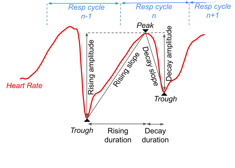
Some features are related to the time of specific points of a respiratory related heart rate oscillation induced by the current respiratory cycle (see figure below for a graphical view of these timepoints/metrics):

• peak_time: Time in seconds of the maximum heart rate during the current respiratory cycle n (usually during inspiration).

• trough_time: Time in seconds of the minimum heart rate of the current respiratory heart rate related oscillation, that could fall in respiratory cycle n (most of the time and usually during expiration) or n+1.

Important note: computing the difference in heart rate within a respiratory cycle provides an absolute measure of RespHRV. However, as discussed by Jerzy Sacha in 2014 (https://doi.org/10.3389/fphys.2013.00306), heart rate variability depends on the average heart rate level. Moreover, since RR intervals and heart rate are non-linearly related (inversely in this case), RespHRV estimated from RR intervals in seconds tends to negatively correlate with average heart rate, whereas RespHRV estimated from heart rate signals (i.e. in bpm) tends to positively correlate with average heart rate. This inverse relationship due to unit choice is nicely illustrated in Figure 1 of the referenced article (Jerzy Sacha, 2014). To avoid misinterpretation due to unit choice and local average heart rate, it is recommended to normalize the absolute RespHRV measurements by the local average heart rate. Accordingly, both absolute and relative RespHRV metrics are provided in the computed features:

• peak_value: (units = those set in compute_resphrv(), default = bpm) Instantaneous heart rate at peak_time, i.e., the maximum heart rate during the ongoing respiratory cycle (usually during inspiration).

• trough_value: (units = those set in compute_resphrv(), default = bpm) Instantaneous heart rate at trough_time, i.e., the minimum heart rate during the ongoing respiratory cycle (usually during expiration). In non-physiological conditions, where the peak time can be delayed toward expiration, this trough value can be measured at a trough time detected in the beginning of the next respiratory cycle n+1.

• min_max_amplitude: (units = those set in compute_resphrv(), default = bpm) Difference between the maximum (max_HR) and minimum (min_HR) heart rate within respiratory cycle n, i.e min_max_amplitude = max_HR - max_HR (see figure below).

• relative_min_max_amplitude: (units = None, but scaled from to 0 to 1) Normalized version of min_max_amplitude, i.e : relative_min_max_amplitude = min_max_amplitude / (max_HR + min_HR)

• rising_amplitude: (units = those set in compute_resphrv(), default = bpm) Difference in heart rate between the maximum of cycle n+1 and the minimum of cycle n (see figure below).

• relative_rising_amplitude: (units = None, but scaled from to 0 to 1) Normalized version of rising_amplitude, i.e : relative_rising_amplitude = rising_amplitude / (max_HRn+1 + min_HRn)

• decay_amplitude: (units = those set in compute_resphrv(), default = bpm) Difference in heart rate between the maximum and the minimum of cycle n. Note that in non-physiological conditions, where the peak time can be delayed toward expiration, the trough value can be measured at a trough time detected in the beginning of the next respiratory cycle n+1, so that the decay_amplitude is computed between a peak value of respiratory cycle n and a trough value detected in respiratory cycle n+1 (see figure below). This corresponds to “how much the heart rate decreases during the current respiratory cycle,” usually at the transition from inspiration to expiration of cycle `n`. Under physiological conditions, this is considered the primary measure of RespHRV, but here it is computed for each cycle.

• relative_decay_amplitude: (units = None, but scaled from to 0 to 1) Normalized version of decay_amplitude, i.e : relative_decay_amplitude = decay_amplitude / (max_HRn + min_HRn)

• rising_duration: (units = s) Duration of the rising_amplitude period, i.e., (peak_time of cycle n – trough_time of cycle n-1).

• decay_duration: (units = s) Duration of the decay_amplitude period, i.e., (trough_time of cycle n – peak_time of cycle n).

• rising_slope: (units = bpm/s by default) Slope of the increase in heart rate, defined as rising_amplitude / rising_duration.

• decay_slope: (units = bpm/s by default) Slope of the decrease in heart rate, defined as decay_amplitude / decay_duration.*

In physiological conditions, we recommend using decay_amplitude as a measure of respiratory heart-rate variability, or even better, its normalized version, relative_decay_amplitude. However, in non-physiological situations— where the heart-rate maximum may be delayed toward the end of the respiratory cycle and/or the RespHRV amplitude is expected to be very low (< 1 bpm)— it is safer to use min_max_amplitude (or relative_min_max_amplitude). This metric simply measures the peak-to-peak heart-rate difference strictly within respiratory cycle n, without considering when within the cycle the peak or trough occurs, this latter point being considered by decay_amplitude or rising_amplitude but becoming (very) noisy when almost no RespHRV exist.

print(f'{resphrv_cycles.shape[1]} computed heart-rate related features in {resphrv_cycles.shape[0]} respiratory cycles, these features being the following :')
pprint(resphrv_cycles.columns.to_list())

14 computed heart-rate related features in 80 respiratory cycles, these features being the following :
['peak_time',
 'trough_time',
 'peak_value',
 'trough_value',
 'min_max_amplitude',
 'relative_min_max_amplitude',
 'rising_amplitude',
 'relative_rising_amplitude',
 'decay_amplitude',
 'relative_decay_amplitude',
 'rising_duration',
 'decay_duration',
 'rising_slope',
 'decay_slope']

Plot RespHRV Amplitude Over Time

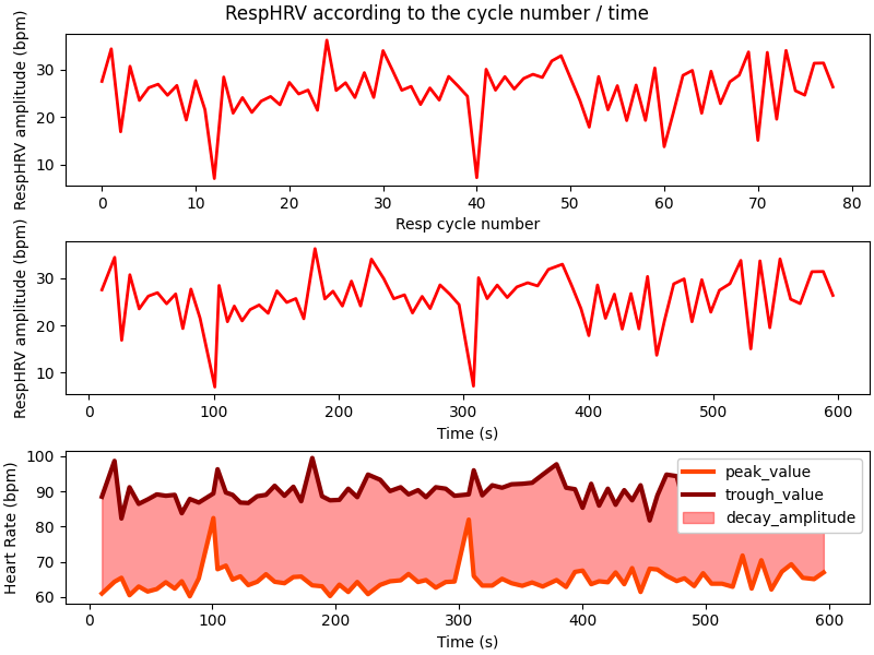
Using the decay_amplitude feature as a marker of cycle-by-cycle RespHRV amplitude, we can plot the dynamics of RespHRV across respiratory cycles or over time (see plot below).

Note that this participant shows an unusually large RespHRV amplitude (~ bpm). For reference, typical values (in bpm) were computed from a sample of N = 3798 cycles pooled from 29 human participants quietly sitting on a chair for 10 minutes:

{‘mean’: 7.47, ‘std’: 7.14, ‘25%’: 2.83, ‘50%’: 5.54, ‘75%’: 10.41, ‘IQR’: 7.58}

fig, axs = plt.subplots(nrows = 3, figsize = (8, 6), constrained_layout = True)
fig.suptitle('RespHRV according to the cycle number / time')

ax = axs[0]
ax.plot(range(resphrv_cycles.shape[0]), resphrv_cycles['decay_amplitude'], color = 'r', lw = 2) # plot decay_amplitude according to cycle number
ax.set_xlabel('Resp cycle number')
ax.set_ylabel('RespHRV amplitude (bpm)')
ax = axs[1]
ax.plot(resphrv_cycles['peak_time'], resphrv_cycles['decay_amplitude'], color = 'r', lw = 2) # plot decay_amplitude according to peak time
ax.set_xlabel('Time (s)')
ax.set_ylabel('RespHRV amplitude (bpm)')

ax = axs[2]
ax.plot(resphrv_cycles['peak_time'], resphrv_cycles['trough_value'], color = 'orangered', label = 'peak_value', lw = 3) # plot trough_value according to peak time
ax.plot(resphrv_cycles['peak_time'], resphrv_cycles['peak_value'], color = 'darkred', label = 'trough_value', lw = 3) # plot peak_value according to peak time
ax.fill_between(resphrv_cycles['peak_time'], resphrv_cycles['trough_value'], resphrv_cycles['peak_value'], color = 'r', alpha = 0.4, label = 'decay_amplitude') # fill between trough_value and peak_value  = RespHRV amplitude
ax.set_xlabel('Time (s)')
ax.set_ylabel('Heart Rate (bpm)')
ax.legend(loc = 'upper right', framealpha = 1)

<matplotlib.legend.Legend object at 0x7390619589d0>

Plot Heart Rate Dynamics According to Respiratory Phase

The function compute_resphrv() internally uses deform_traces_to_cycle_template() to deform the instantaneous heart rate vector according to inspiratory/expiratory time points (see Cyclic Deformation Tutorial for more information about cyclical deformation).

As a result, compute_resphrv() returns cyclic_cardiac_rate, a 2D NumPy array of shape (n_resp_cycles, points_per_cycle). Each cell of this array contains a heart rate value, expressed in the units set in compute_resphrv() (default = bpm).

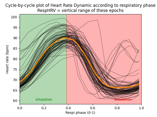
This matrix provides a detailed view of heart rate dynamics at each phase point of every respiratory cycle. Specifically, points_per_cycle defines the number of respiratory phase points to which the heart rate is reinterpolated.

Using this representation, one can plot the cycle-by-cycle dynamics of heart rate during each respiratory cycle (shown as overlapping black traces in the figure below) along with the average heart rate dynamics (shown as the thick orange trace), relative to the normalized respiratory phase (normalized from 0 to 1, but it can also be expressed from 0 to 2π or –π to π).

cycle_ratio = resp_cycles['cycle_ratio'].mean() # get the average cycle ratio, internally used by physio.compute_resphrv as the segment_ratios, if two_segment = True

one_cycle = np.arange(points_per_cycle) / points_per_cycle # compute normalized respiratory phase vector
fig, ax = plt.subplots()
ax.plot(one_cycle, cyclic_cardiac_rate.T, color='k', alpha=.3) # plot heart rate dynamic for each cycle, overlapped, in black, according to resp phase
ax.plot(one_cycle, np.mean(cyclic_cardiac_rate, axis=0), color='darkorange', lw=3) # # plot average heart rate dynamic, in orange, according to resp phase. The mean is computed along axis 0 meaning along the resp cycles axis.
ax.axvspan(0, cycle_ratio, color='g', alpha=0.3) # plot a vertical green span from 0 to the mean cycle_ratio (meaning the mean normalized transition from inspi to expi) to display inspiration period
ax.axvspan(cycle_ratio, 1, color='r', alpha=0.3) # plot a vertical red span from the mean cycle_ratio to 1 to display expiration period
ax.set_xlabel('Respi phase (0-1)')
ax.set_ylabel('Heart rate (bpm)')
ax.set_xlim(0, 1)
ax.text(0.2, 60, 'inhalation', ha='center', color='g')
ax.text(0.85, 60, 'exhalation', ha='center', color='r')
ax.set_title('Cycle-by-cycle plot of Heart Rate Dynamic according to respiratory phase\nRespHRV = vertical range of these epochs')


plt.show()

Plot heart rate dynamic according to time and respiratory phase

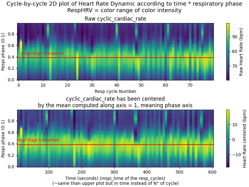
A nice way of seeing RespHRV can be a 2D plot showing evolution along time / resp cycles of the heart rate dynamics along each respiratory cycle

fig, axs = plt.subplots(nrows = 2, figsize = (8, 6), constrained_layout = True, sharex = False)
fig.suptitle('Cycle-by-cycle 2D plot of Heart Rate Dynamic according to time * respiratory phase\nRespHRV = color range of color intensity', fontsize=  13)

ax = axs[0]
im = ax.pcolormesh(range(resp_cycles.shape[0]), one_cycle, cyclic_cardiac_rate.T, cmap = 'viridis') # plot 2D view of heart rate dynamic for each cycle (in abscissa) and each phase point (in ordinate)
fig.colorbar(im, ax=ax).set_label('Raw Heart Rate (bpm)')
ax.set_title('Raw cyclic_cardiac_rate')
ax.set_xlabel('Resp cycle Number')

ax = axs[1]
cyclic_cardiac_rate_centered = cyclic_cardiac_rate - np.mean(cyclic_cardiac_rate, axis = 1)[:,None] # Center each heart rate epoch by subtracting to them the mean of each one
# This can be useful to focus just on heart rate by-cycle variations and remove slow heart rate drifts than can bother the viewing of RespHRV

im = ax.pcolormesh(resp_cycles['inspi_time'], one_cycle, cyclic_cardiac_rate_centered.T, cmap = 'viridis') # plot 2D view of heart rate dynamic for each cycle (in abscissa) and each phase point (in ordinate)
fig.colorbar(im, ax=ax).set_label('Heart Rate centered (bpm)')
ax.set_title('cyclic_cardiac_rate has been centered\nby the mean computed along axis = 1, meaning phase axis')
ax.set_xlabel('Time (seconds) (inspi_time of the resp_cycles)\n(~same than upper plot but in time instead of N° of cycle)')

for ax in axs:
    ax.set_ylabel('Respi phase (0-1)')
    ax.axhline(cycle_ratio, color = 'r') # plot a horizontal red line at the mean cycle_ratio
    ax.text(1, cycle_ratio + 0.05, 'Inspi-Expi transition', ha='left', color='r')

plt.show()

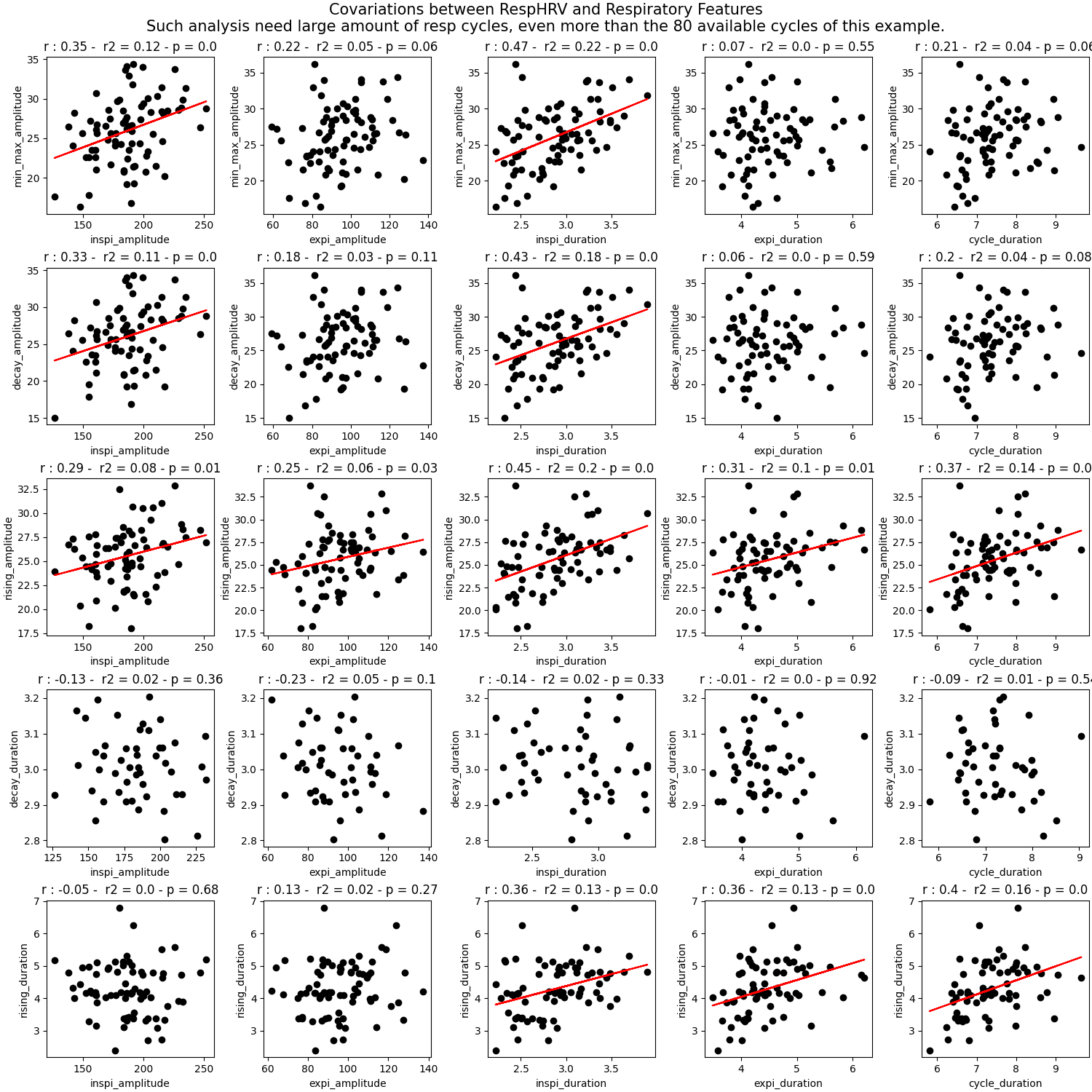
Explore Covariations Between RespHRV and Respiratory Features

resp_cycles and resphrv_cycles contain the same number of rows, since they describe respiratory and heart rate features for each respiratory cycle (nrows = n_cycles).

This makes it possible to analyze covariations between cycle-by-cycle respiratory features and RespHRV features.

For such an analysis, ensure that your dataset includes a sufficient number of respiratory cycles and/or enough variation in respiratory features or regimes. Otherwise, there may not be enough variability to meaningfully explore the covariations.

In this example, only 5 minutes of respiration and ECG signals were recorded in a quiet resting state. Therefore, variability and the number of cycles are limited. Nevertheless, we perform such an analysis here for demonstration purposes.

Note that a well-established statistical association between respiratory cycle duration and RespHRV amplitude is expected, as shown by Hirsh & Bishop (1981) in Respiratory sinus arrhythmia in humans: how breathing pattern modulates heart rate (DOI: 10.1152/ajpheart.1981.241.4.H620).

In general, the longer the respiratory cycle duration (i.e., the lower the respiratory rate), the greater the RespHRV amplitude (i.e., higher decay_amplitude / rising_amplitude / min_max_amplitude), up to a certain limit (~7.2 cycles per minute / 0.11 Hz / 8.5 seconds per cycle). Below a breathing rate of 0.11 Hz, no further association is expected.

Thus, when the respiratory rate decreases for experimental reasons, an accompanying increase in RespHRV amplitude is “normal.” This is partly why Hirsh & Bishop (1981) proposed “normalizing” RespHRV amplitude by respiratory rate in order to theoretically isolate the true effect of an experimental manipulation on RespHRV amplitude, independent of the influence of respiratory rate itself.

Using the cycle-by-cycle analysis of both respiration and heart rate (resp_cycles and resphrv_cycles) provided by physio may allow users to normalize RespHRV amplitude by respiratory rate, for example by applying a linear mixed-effects model that adjusts for respiratory rate, or the methods described in Hirsh & Bishop (1981).

alpha = 0.05 # regression line will be plotted if the regression fit p-value is lower than this alpha threshold

# define a function to filter outliers
def filter_outliers(x, y):
   _factor = 3

   med, mad = physio.compute_median_mad(x[~np.isnan(x)])
   x_keep = (x >= med - _factor * mad) & (x <= med + _factor * mad)

   med, mad = physio.compute_median_mad(y[~np.isnan(y)])
   y_keep = (y >= med - _factor * mad) & (y <= med + _factor * mad)

   and_keep = x_keep & y_keep
   return x[and_keep], y[and_keep]

resp_sel_metrics = ['inspi_amplitude','expi_amplitude','inspi_duration','expi_duration','cycle_duration'] # select some respiratory features to study
resphrv_sel_metrics = ['min_max_amplitude','decay_amplitude','rising_amplitude','decay_duration','rising_duration'] # select some RespHRV features to study

nrows = len(resphrv_sel_metrics)
ncols = len(resp_sel_metrics)

fig, axs = plt.subplots(nrows, ncols, figsize = (ncols * 3, nrows * 3), constrained_layout = True)
fig.suptitle(f'Covariations between RespHRV and Respiratory Features\nSuch analysis need large amount of resp cycles, even more than the {resp_cycles.shape[0]} available cycles of this example.', fontsize = 15)

for c, resp_metric in enumerate(resp_sel_metrics):
  for r, resphrv_metric in enumerate(resphrv_sel_metrics):
    ax = axs[r,c]

    x, y = filter_outliers(resp_cycles[resp_metric].values, resphrv_cycles[resphrv_metric].values) # filter paired outliers

    res = stats.linregress(x,y) # linear regression from scipy.stats

    ax.set_title(f'r : {round(res.rvalue,2)} -  r2 = {round(res.rvalue**2,2)} - p = {round(res.pvalue, 2)}')
    if res.pvalue < alpha: # plot regression line if p-value < alpha
      ax.plot(x, res.intercept + res.slope*x, color = 'r')
    ax.scatter(x, y, color = 'k')
    ax.set_ylabel(resphrv_metric)
    ax.set_xlabel(resp_metric)

plt.show()