ECG tutorial

import numpy as np
import matplotlib.pyplot as plt
from pathlib import Path
from pprint import pprint

import physio

Detect ECG R peaks. The faster way: using parameter_preset.

The fastest way to process ECG with physio is to use compute_ecg() which is a high-level wrapper function that simplifies ECG signal analysis. To use this function, you must provide:

• raw_ecg : the raw ECG signal as a NumPy array

• srate : the sampling rate of the ECG signal

• parameter_preset : a string specifying the type of ECG data, which determines the set of parameters used for processing. Can be one of: human_ecg or rat_ecg.

When called, compute_ecg() performs the following:

• Preprocesses the ECG signal (returns a NumPy array: ecg). By default, ecg is normalized.

• Detects R peaks (returns a pd.DataFrame: ecg_peaks)

Warning: The orientation of the raw_ecg trace is important (multiply it by -1 for reversing it if necessary). R peaks must point upward for the highest probability of detection by compute_ecg(). Sometimes the R and S peaks of the QRS complex are equivalent, so orientation does not matter, because either the R or S peak will be detected and used to mark heartbeats.

For this tutorial, we will use an internal file already stored in NumPy format for demonstration purposes.

raw_ecg = np.load('ecg1.npy') # load ecg
srate = 1000. # our example signals have been recorded at 1000 Hz

times = np.arange(raw_ecg.size) / srate # build time vector

ecg, ecg_peaks = physio.compute_ecg(raw_ecg, srate, parameter_preset='human_ecg') # set 'human_ecg' as preset because example ecg is from human

# ecg_peaks is a dataframe containing 2 columns : 1) the indices of detection and 2) the times in seconds of detections of the R peaks
print(ecg_peaks)

r_peak_ind = ecg_peaks['peak_index'].values # get index of detected R peaks

linewidth = 0.8
fig, axs = plt.subplots(nrows=2, sharex=True)
ax = axs[0]
ax.plot(times, raw_ecg, lw = linewidth)
ax.scatter(times[r_peak_ind], raw_ecg[r_peak_ind], color="#C3CB22", label = 'R peak')
ax.set_ylim(0.0145, 0.0175)
ax.set_ylabel('Amplitude (V)')
ax.set_title('R peak detection, plotted on raw ECG')
ax.legend(loc = 'upper right')

ax = axs[1]
ax.plot(times, ecg, lw = linewidth)
ax.scatter(times[r_peak_ind], ecg[r_peak_ind], color='#A8AE27', label = 'R peak')
ax.set_ylabel('Amplitude (AU)')
ax.set_title('R peak detection, plotted on preprocessed ECG')
ax.legend(loc = 'upper right')

ax.set_xlabel('Time (s)')
ax.set_xlim(95, 125)

     peak_index  peak_time
0           318      0.318
1           899      0.899
2          1470      1.470
3          2032      2.032
4          2589      2.589
..          ...        ...
403      296754    296.754
404      297337    297.337
405      297917    297.917
406      298520    298.520
407      299237    299.237

[408 rows x 2 columns]

(95.0, 125.0)

What is parameter_preset ?

Using parameter_preset tells compute_ecg() to process ECG according to a predefined set of parameters already optimized by physio.

To get an idea of the default parameters used in parameter_preset, you can call get_ecg_parameters().

Here is an example showing the set of parameters applied in the case of a human ECG signal.

parameters = physio.get_ecg_parameters('human_ecg') # parameters is a nested dictionary of parameters used at each processing step.
pprint(parameters) # pprint to "pretty print"

{'peak_clean': {'min_interval_ms': 400.0},
 'peak_detection': {'exclude_sweep_ms': 4.0, 'thresh': 'auto'},
 'preprocess': {'band': [5.0, 45.0],
                'ftype': 'bessel',
                'normalize': True,
                'order': 5}}

Tuning parameters if unsatisfied

Variability during data acquisition (subject, acquisition system) can affect the recorded ECG signal. Such variability may make some predefined parameters of physio inappropriate.

In this situation, you can tune certain parameters by re-assigning values to the keys of the parameters dictionary. You may also tune multiple parameters at once if necessary. To fine-tune parameters properly, a good understanding of each parameter’s role is required. For this reason, we have dedicated a whole section to this topic — see the “Parameters” section.

For example, here we modify 3 parameters:

• the amplitude above which R peak can be detected

• the minimum possible duration in milliseconds between two consecutive R peaks

• the frequency band of the filter

# let's change 3 parameters in the nested structure ...
parameters['peak_detection']['thresh'] = 4 # at the key "peak_detection" and the sub-key "thresh", the default values is 'auto', meaning an automatically computed threshold of detection. Here we replace it to 4 to allow for peaks at least higher than 4 to be detected.
parameters['peak_clean']['min_interval_ms'] = 300 # at the key "peak_clean" and the sub-key "min_interval_ms", the default values is 400 milliseconds. Here we replace it to 300 to allow smaller RR intervals to be detected, meaning faster heart rate.
parameters['preprocess']['band'] = [2., 25.] # at the key "preprocess" and the sub-key "band", the default values is [5., 45.] Hz. Here we replace it to [2., 40.] Hz to target a slightly lower frequency band.
pprint(parameters)

ecg, ecg_peaks = physio.compute_ecg(raw_ecg, srate, parameters=parameters) # preset_parameters = None in this case, because parameters is now explicitly defined

print(ecg_peaks)

r_peak_ind = ecg_peaks['peak_index'].values # get index of detected R peaks

fig, ax = plt.subplots()
ax.plot(times, ecg)
ax.scatter(times[r_peak_ind], ecg[r_peak_ind], marker='o', color='magenta')
ax.set_ylabel('Amplitude (AU)')
ax.set_title('R peak detection, plotted on preprocessed ECG')
ax.set_xlabel('Time (s)')
ax.set_xlim(95, 125)

{'peak_clean': {'min_interval_ms': 300},
 'peak_detection': {'exclude_sweep_ms': 4.0, 'thresh': 4},
 'preprocess': {'band': [2.0, 25.0],
                'ftype': 'bessel',
                'normalize': True,
                'order': 5}}
     peak_index  peak_time
0           316      0.316
1           896      0.896
2          1467      1.467
3          2029      2.029
4          2586      2.586
..          ...        ...
403      296751    296.751
404      297333    297.333
405      297914    297.914
406      298517    298.517
407      299234    299.234

[408 rows x 2 columns]

(95.0, 125.0)

Heart Rate Variability metrics (time-domain)

compute_ecg_metrics() is a high-level wrapper function that computes time-domain Heart Rate Variability (HRV) metrics from previously detected R peaks (ecg_peaks). To use this function, you must provide the previously detected R peaks, ecg_peaks:

• ecg_peaks: pd.DataFrame, output of the function compute_ecg()

• min_interval_ms: float, minimum RR interval in milliseconds (optional, default = 500 ms)

• max_interval_ms: float, maximum RR interval in milliseconds (optional, default = 2000 ms)

When called, compute_ecg_metrics() performs the following:

• Computes the time differences between successive RR intervals.

• Cleans the RR intervals according to min_interval_ms and max_interval_ms.

• Computes HRV time-domain metrics from the cleaned RR intervals.

Computed metrics are:

• HRV_Mean: (units = ms for milliseconds) Mean of the RR intervals. Note that the “HRV” terminology can be misleading here, as it is inspired by other toolboxes and does not strictly measure variability, but rather an estimation of the position in the distribution.

• HRV_SD: (units = ms) Standard deviation of the RR intervals.

• HRV_Median: (units = ms) Median of the RR intervals. As RR interval distributions are rarely normal, we recommend using HRV_Median instead of HRV_Mean for estimating central tendency.

• HRV_Mad: (units = ms) Median absolute deviation (MAD) of the RR intervals. HRV_Mad is more robust to outliers than HRV_SD and is therefore recommended for variability estimation (see 10.1016/j.jesp.2013.03.013).

• HRV_CV: (units = AU) Coefficient of variation of RR intervals = HRV_SD / HRV_Mean. This provides a standardized measure of variability, reducing the effect of the central tendency on dispersion.

• HRV_MCV: (units = AU) “MAD” coefficient of variation = HRV_Mad / HRV_Median. This robust measure standardizes variability while being less sensitive to outliers.

• HRV_Asymmetry: (units = ms) Difference between HRV_Mean and HRV_Median. This provides a simple measure of skewness or non-normality in the RR interval distribution and can highlight potential outlier effects.

• HRV_RMSSD: (units = ms) Root mean square of successive differences (RMSSD). RMSSD is calculated as the square root of the mean of the squared differences between successive RR intervals. Conceptually, it is similar to a second derivative of the RR intervals (if RR intervals are considered as a first derivative). RMSSD is very sensitive to outliers, which can artificially increase its value.

Some of these metrics can be visualized on the RR interval distribution below, which provides a simple way to identify potential outliers in the detection.

Note that the impact of outliers in R peak detection on HRV metrics—often due to poor ECG quality—can be mitigated in three ways:

1. By using optimal parameters during R peak detection with compute_ecg()

2. By setting appropriate min_interval_ms and max_interval_ms when using compute_ecg_metrics()

3. By interpreting results using robust metrics such as HRV_Median, HRV_Mad, or HRV_MCV

While these three steps can reduce the impact of outliers, careful ECG data recording is no substitute for quality optimization.

ecg_metrics = physio.compute_ecg_metrics(ecg_peaks, min_interval_ms=500., max_interval_ms=2000) # ecg_metrics = a pd.Series containing HRV time domain results. Here we set 500 to 2000 ms as a normal range of RRi for a human quietly sitting on a chair.

peak_times = ecg_peaks['peak_time'].values # get R peak times of detection
rri_s = np.diff(peak_times) # compute RR intervals in seconds
rri_ms = rri_s * 1000 # seconds to milliseconds

fig, ax = plt.subplots()
ax.hist(rri_ms, bins=np.arange(500, 1400, 25), edgecolor = 'k') # plot distribution of RR intervals
ax.axvline(ecg_metrics['HRV_Mean'], color='orange', label='Mean RRi') # vertical line at the mean RRi
ax.axvline(ecg_metrics['HRV_Median'], color='violet', label='Median RRi') # vertical line at the median RRi
ax.axvspan(ecg_metrics['HRV_Median'] - 2*ecg_metrics['HRV_Mad'], ecg_metrics['HRV_Median'] + 2*ecg_metrics['HRV_Mad'], color = 'orange', alpha = 0.1, label = 'Median +/- 2 * Median Absolute Deviation') # vertical span at the med + 2*mad
ax.axvspan(ecg_metrics['HRV_Mean'] - 2*ecg_metrics['HRV_SD'], ecg_metrics['HRV_Mean'] + 2*ecg_metrics['HRV_SD'], color = 'violet', alpha = 0.1, label = 'Mean +/- 2 * Standard-Deviation') # vertical span at the mean + 2*sd
ax.set_xlabel('RR interval (ms)')
ax.set_ylabel('Count')
ax.set_ylim(-5, 90)
ax.legend(loc = 'upper center', ncols = 2)
ax.set_title('Distribution or RR intervals + Heart Rate Variability metrics')
print(ecg_metrics)

HRV_Mean         734.442260
HRV_SD           145.915717
HRV_Median       678.000000
HRV_Mad          115.642973
HRV_CV             0.198676
HRV_MCV            0.170565
HRV_Asymmetry    -56.442260
HRV_RMSSD        103.558543
dtype: float64

Heart Rate Variability metrics (frequency-domain)

compute_hrv_psd() is a high-level wrapper function that computes frequency-domain Heart Rate Variability (HRV) metrics from previously detected R peaks (ecg_peaks).

To use this function, you must provide the previously detected R peaks (ecg_peaks) along with other optional parameters:

• ecg_peaks: pd.DataFrame, output of the function compute_ecg()

• sample_rate: float, sampling frequency of the reconstructed instantaneous heart rate (IHR) vector through interpolation (optional, default = 100 Hz). This vector is used internally by the function, so this parameter usually does not need adjustment. 100 Hz works well for both humans and rodents.

• limits: list or None, range in the chosen units for removing outliers (e.g., [30, 200] to exclude bpm values outside this range). Default is None, meaning no cleaning.

• units: str (‘bpm’, ‘Hz’, ‘ms’, ‘s’), sets the output units (default = ‘bpm’).

• frequency_bands: dict. Example: {‘lf’: (0.04, 0.15), ‘hf’: (0.15, 0.4)} (default). Frequency band names and ranges are defined using this dictionary. You may explore lower frequencies if your signal duration is sufficient.

• window_s: float, default = 250 seconds. Duration of the window used for power spectral density estimation via Welch’s method. It must be long enough to cover at least 5 cycles of the lowest frequency you wish to analyze; otherwise, compute_hrv_psd() will raise an error.

• interpolation_kind: str (‘linear’ or ‘cubic’). Method to reconstruct the IHR vector. Linear interpolation uses straight lines, while cubic interpolation produces smooth curves. Default is “cubic”. The choice affects signal smoothness and dynamics, and therefore influences the power spectrum due to differences in harmonic content.

When called, compute_hrv_psd() performs the following:

• Compute an instantaneous heart rate vector from ecg peaks and compute a Fourier transform using Welch method (returns two NumPy arrays: psd_freqs and psd giving frequency vector and power vector, respectively).

• Compute HRV frequency metrics by getting power for each frequency band using trapezoïdal rule (returns a pd.Series: psd_metrics, with units in the set units² / Hz)

frequency_bands = {'lf': (0.04, .15), 'hf' : (0.15, .4)} # set classical cutoffs of low and high frequency bands, in a dictionnary
psd_freqs, psd, psd_metrics = physio.compute_hrv_psd(ecg_peaks=ecg_peaks, frequency_bands=frequency_bands)

print(psd_metrics)
fig, ax = plt.subplots()
ax.plot(psd_freqs, psd)
colors = {'lf': '#B8860B', 'hf' : '#D2691E'}
for name, freq_band in frequency_bands.items():
    ax.axvspan(*freq_band, alpha=0.1, color=colors[name], label=f'{name} : {round(psd_metrics[name], 2)}') # plot one vertical span for each frequency band
ax.set_xlim(0, 0.6)
ax.set_xlabel('Frequency (Hz)')
ax.set_ylabel('Power Spectral Density')
ax.legend(loc = 'upper right')
ax.set_title('HRV Power Spectral Density\n-> Frequency-Domain metrics')

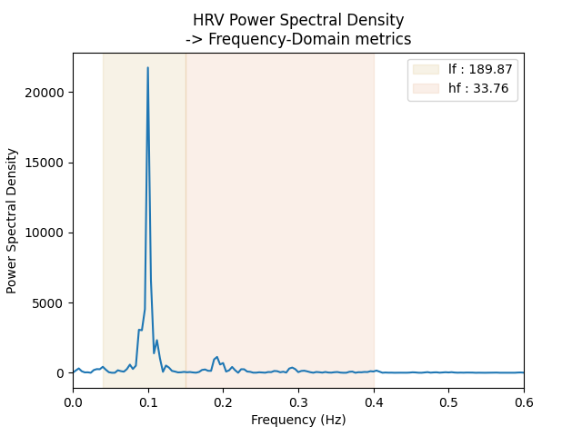
lf    189.868381
hf     33.763727
dtype: float64

Text(0.5, 1.0, 'HRV Power Spectral Density\n-> Frequency-Domain metrics')

From R Peaks to Instantaneous Heart Rate

Computing HRV metrics in the frequency domain first requires computing an instantaneous heart rate vector, regularly sampled. You may want to explore this reconstructed time series.

This can be done using the RR intervals (RRi), which are naturally a time series. To move from time units (RR interval duration) to frequency, recall that Frequency (F) = 1 / T, where T is a period such as RRi.

Concerning heart rate, the standard is not to count how many heartbeats we have per second, but per minute. The idea is to compute, for each RRi, how many of them would occur in one minute.

The formula is the following:

• Heart rate [bpm] = 60 / RRi (s)

where “bpm” stands for “beats per minute” and “s” for “seconds”.

However, most toolboxes work with “RRi in ms,” while heart rate in bpm is often more intuitive:

• With bpm units, an increase in the time series means a heart rate acceleration.

• With ms units, an increase in the time series means a heart rate deceleration.

That said, feel free to use whichever units you prefer (bpm or ms).

The physio module provides the function compute_instantaneous_rate() to obtain instantaneous heart rate (in bpm) or heart period (in ms) from previously detected R peaks using interpolation.

To use this function, you must provide:

• ecg_peaks : pd.DataFrame, output of compute_ecg()

• new_times : np.array, the regularly sampled time series on which to compute instantaneous heart rate. This can be the ECG time vector, or a down-sampled version to reduce computation.

• limits : list or None, range in the chosen units for removing outliers (e.g. [30, 200] to exclude bpm outside this range). Default is None, meaning no cleaning.

• units : str (‘bpm’ / ‘Hz’ / ‘ms’ / ‘s’), sets the output units (default = ‘bpm’).

• interpolation_kind : str (‘linear’ or ‘cubic’). Linear interpolation uses straight lines, while cubic interpolation uses smooth curves. Default is “linear”.

When called, compute_ecg() performs the following:

• Converts units according to the “units” parameter

• Removes outliers if limits are provided

• Interpolates the time series according to the new_times vector

Let’s use it.

new_times = times[::10] # time vector used for interpolation, here the time vector of the raw ECG but down sampeld 10 times
instantaneous_heart_rate = physio.compute_instantaneous_rate(
    ecg_peaks,
    new_times,
    limits=None,
    units='bpm', # units in beats per minute
    interpolation_kind='linear',
)
instantaneous_heart_period = physio.compute_instantaneous_rate(
    ecg_peaks,
    new_times,
    limits=None,
    units='ms', # units in milliseconds
    interpolation_kind='linear',
)

fig, axs = plt.subplots(nrows=2, sharex=True)
fig.suptitle('From R peaks to Instantaneous Heart Rate')
ax = axs[0]
ax.plot(new_times, instantaneous_heart_rate)
ax.set_ylabel('Heart Rate (bpm)')
ax = axs[1]
ax.plot(new_times, instantaneous_heart_period)
ax.set_ylabel('Heart Period (ms)')
ax.set_xlabel('Time (s)')
ax.set_xlim(100, 150)

(100.0, 150.0)